(Part I of this post is here)
Let ![p(n)]() denote the partition function, which describes the number of ways to write
denote the partition function, which describes the number of ways to write ![n]() as a sum of positive integers, ignoring order. In 1918 Hardy and Ramanujan proved that
as a sum of positive integers, ignoring order. In 1918 Hardy and Ramanujan proved that ![p(n)]() is given asymptotically by
is given asymptotically by
![\displaystyle p(n) \approx \frac{1}{4n \sqrt{3}} \exp \left( \pi \sqrt{ \frac{2n}{3} } \right)]() .
.
This is a major plot point in the new Ramanujan movie, where Ramanujan conjectures this result and MacMahon challenges him by agreeing to compute ![p(200)]() and comparing it to what this approximation gives. In this post I’d like to describe how one might go about conjecturing this result up to a multiplicative constant; proving it is much harder.
and comparing it to what this approximation gives. In this post I’d like to describe how one might go about conjecturing this result up to a multiplicative constant; proving it is much harder.
Verification
MacMahon computed ![p(200)]() using a recursion for
using a recursion for ![p(n)]() implied by the pentagonal number theorem, which makes it feasible to compute
implied by the pentagonal number theorem, which makes it feasible to compute ![p(200)]() by hand. Instead of doing it by hand I asked WolframAlpha, which gives
by hand. Instead of doing it by hand I asked WolframAlpha, which gives
![\displaystyle p(200) = 3972999029388 \approx 3.973 \times 10^{12}]()
whereas the asymptotic formula gives
![\displaystyle \frac{1}{800 \sqrt{3}} \exp \left( \pi \sqrt{ \frac{400}{3} } \right) \approx 4.100 \times 10^{12}]() .
.
Ramanujan is shown getting closer than this in the movie, presumably using a more precise asymptotic.
How might we conjecture such a result? In general, a very powerful method for figuring out the growth rate of a sequence ![a_n]() is to associate to it the generating function
is to associate to it the generating function
![\displaystyle A(z) = \sum_{n=0}^{\infty} a_n z^n]()
and relate the behavior of ![A(z)]() , often for complex values of
, often for complex values of ![z]() , to the behavior of
, to the behavior of ![a_n]() . The most comprehensive resource I know for descriptions both of how to write down generating functions and to analyze them for asymptotic behavior is Flajolet and Sedgewick’s Analytic Combinatorics, and the rest of this post will follow that book’s lead closely.
. The most comprehensive resource I know for descriptions both of how to write down generating functions and to analyze them for asymptotic behavior is Flajolet and Sedgewick’s Analytic Combinatorics, and the rest of this post will follow that book’s lead closely.
The meromorphic case
The generating function strategy is easiest to carry out in the case that ![A(z)]() is meromorphic (for example, if it’s rational); in that case the asymptotic growth of
is meromorphic (for example, if it’s rational); in that case the asymptotic growth of ![a_n]() is controlled by the behavior of
is controlled by the behavior of ![a(z)]() near the pole (or poles) closest to the origin. For rational
near the pole (or poles) closest to the origin. For rational ![A(z)]() this is particularly simple and just a matter of looking at the partial fraction decomposition.
this is particularly simple and just a matter of looking at the partial fraction decomposition.
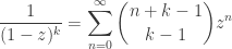
Example.The generating function for the sequence ![p_k(n)]() of partitions into parts of size at most
of partitions into parts of size at most ![k]() is the rational function
is the rational function
![\displaystyle P_k(z) = \frac{1}{(1 - z) \dots (1 - z^k)}]()
whose most important pole is at ![z = 1]() and of order
and of order ![k]() , and whose other poles are at the
, and whose other poles are at the ![k^{th}]() roots of unity, and of order at most
roots of unity, and of order at most ![\frac{k}{2}]() . We can factor
. We can factor ![P_k(z)]() as
as
![\displaystyle P_k(z) = \frac{1}{(1 - z)^k} \left( \frac{1}{(1 + z)(1 + z + z^2) \dots (1 + z + \dots + z^{k-1})} \right)]()
which gives, upon substituting ![z = 1]() , that the partial fraction decomposition begins
, that the partial fraction decomposition begins
![\displaystyle P_k(z) = \frac{1}{k! (1 - z)^k} + \text{lower terms}]()
and hence, using the fact that
![\displaystyle \frac{1}{(1 - z)^k} = \sum_{n=0}^{\infty} {n+k-1 \choose k-1} z^n]()
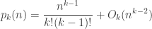
we conclude that ![p_k(n)]() is asymptotically
is asymptotically
![\displaystyle p_k(n) = \frac{n^{k-1}}{k! (k-1)!} + O_k(n^{k-2})]() .
.
We ignored all of the other terms in the partial fraction decomposition to get this estimate, so there’s no reason to expect it to be particularly accurate unless ![n]() is fairly large compared to
is fairly large compared to ![k]() . Nonetheless, let’s see if we can learn anything from it about how big we should expect the partition function
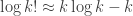
. Nonetheless, let’s see if we can learn anything from it about how big we should expect the partition function ![p(n)]() itself to be. Taking logs and using the rough form
itself to be. Taking logs and using the rough form ![\log k! \approx k \log k - k]() of Stirling’s approximation gives
of Stirling’s approximation gives
![\displaystyle \log p_k(n) \approx k \log n - 2k \log k + 2k]()
and substituting ![k = n^r]() for some
for some ![0 < r < 1]() gives
gives
![\displaystyle \log p_{n^r}(n) \approx \left( n^r - 2r n^r \right) \log n + 2n^r]() .
.
If ![r > \frac{1}{2}]() then this quantity is negative; at this point we’re clearly not in the regime where this approximation is accurate. If
then this quantity is negative; at this point we’re clearly not in the regime where this approximation is accurate. If ![r < \frac{1}{2}]() then the first term dominates and we get something that grows like
then the first term dominates and we get something that grows like ![n^r \log n]() . But if
. But if ![r = \frac{1}{2}]() then the first term vanishes and we get
then the first term vanishes and we get
![\displaystyle \log p_{\sqrt{n}}(n) \approx 2 \sqrt{n}]() .
.
This is at least qualitatively the correct behavior for ![\log p(n)]() , and the multiplicative constant isn’t so off either: the correct value is
, and the multiplicative constant isn’t so off either: the correct value is ![\pi \sqrt{\frac{2}{3}} \approx 2.565]() .
.
Example. A weak order is like a total order, but with ties: for example, it describes a possible outcome of a horse race. Let ![w_n]() denote the number of weak orders of
denote the number of weak orders of ![n]() elements (the ordered Bell numbers, or Fubini numbers). General techniques described in Flajolet and Sedgewick can be used to show that
elements (the ordered Bell numbers, or Fubini numbers). General techniques described in Flajolet and Sedgewick can be used to show that ![w_n]() has exponential generating function
has exponential generating function
![\displaystyle W(z) = \sum_{n=0}^{\infty} \frac{w_n}{n!} z^n = \frac{1}{2 - e^z}]()
(which should be parsed as ![\frac{1}{1 - (e^z - 1)}]() ; loosely speaking, this corresponds to a description of the combinatorial species of weak orders as the species of “lists of nonempty sets”). This is a meromorphic function with poles at
; loosely speaking, this corresponds to a description of the combinatorial species of weak orders as the species of “lists of nonempty sets”). This is a meromorphic function with poles at ![z = \log 2 + 2 \pi i k, k \in \mathbb{Z}]() . The unique pole closest to the origin is at
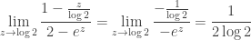
. The unique pole closest to the origin is at ![z = \log 2]() , and we can compute using l’Hopital’s rule that
, and we can compute using l’Hopital’s rule that
![\displaystyle \lim_{z \to \log 2} \frac{1 - \frac{z}{\log 2}}{2 - e^z} = \lim_{z \to \log 2} \frac{- \frac{1}{\log 2}}{-e^z} = \frac{1}{2 \log 2}]()
and hence the partial fraction decomposition of ![F(z)]() begins
begins
![\displaystyle W(z) = \frac{1}{2 \log 2 \left( 1 - \frac{z}{\log 2} \right)} + \text{lower terms}]()
which gives the asymptotic
![\displaystyle w_n = \frac{n!}{2 (\log 2)^{n+1}} + O \left( \frac{n!}{|\log 2 + 2 \pi i|^n} \right)]()
Curiously, the error in the above approximation has some funny quasi-periodic behavior corresponding to the arguments of the next most relevant poles, at ![\log 2 \pm 2 \pi i]() .
.
The saddle point bound
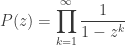
However, understanding meromorphic functions is not enough to handle the case of partitions, where the relevant generating function is
![\displaystyle P(z) = \prod_{k=1}^{\infty} \frac{1}{1 - z^k}]() .
.
This function is holomorphic inside the unit disk but has essential singularities at every root of unity, and to handle it we will need a more powerful method known as the saddle point method, which is beautifully explained with pictures both in Flajolet and Sedgewick and in these slides, and concisely explained in these notes by Jacques Verstraete.
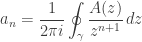
The starting point is that we can recover the coefficients ![a_n]() of a generating function
of a generating function ![A(z) = \sum a_n z^n]() using the Cauchy integral formula, which gives
using the Cauchy integral formula, which gives
![\displaystyle a_n = \frac{1}{2 \pi i} \oint_{\gamma} \frac{A(z)}{z^{n+1}} \, dz]()
where ![\gamma]() is a closed contour in
is a closed contour in ![\mathbb{C}]() with winding number
with winding number ![1]() around the origin and such that ;
around the origin and such that ;![A(z)]() is holomorphic in an open disk containing
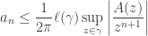
is holomorphic in an open disk containing ![\gamma]() . This integral can be straightforwardly bounded by the product of the length of
. This integral can be straightforwardly bounded by the product of the length of ![\gamma]() , denoted
, denoted ![\ell(\gamma)]() , and the maximum value that
, and the maximum value that ![\frac{A(z)}{z^{n+1}}]() takes on it, which gives
takes on it, which gives
![\displaystyle a_n \le \frac{1}{2 \pi} \ell(\gamma) \sup_{z \in \gamma} \left| \frac{A(z)}{z^{n+1}} \right|]() .
.
From here, the name of the game is to attempt to pick ![\gamma]() such that this bound is as good as possible. For example, if we pick
such that this bound is as good as possible. For example, if we pick ![\gamma]() to be the circle of radius
to be the circle of radius ![r]() , then
, then ![\ell(\gamma) = 2 \pi r]() . If
. If ![A(z)]() has nonnegative coefficients, which will always be the case in combinatorial applications, then
has nonnegative coefficients, which will always be the case in combinatorial applications, then ![\frac{A(z)}{z}]() will take its maximum value when
will take its maximum value when ![z = r]() , which gives the saddle point bound
, which gives the saddle point bound
![\displaystyle a_n \le \frac{A(r)}{r^n}]()
as long as ![A(z)]() is holomorphic in an open disk of radius greater than
is holomorphic in an open disk of radius greater than ![r]() . Strictly speaking, this bound doesn’t require any complex analysis to prove: if
. Strictly speaking, this bound doesn’t require any complex analysis to prove: if ![A(z)]() has nonnegative coefficients and
has nonnegative coefficients and ![A(r)]() converges then for
converges then for ![r \ge 0]() we clearly have
we clearly have
![\displaystyle A(r) = \sum_{n=0}^{\infty} a_n r^n \ge a_n r^n]() .
.
But later we will actually use some complex analysis to improve the saddle point bound to an estimate.
The saddle point bound gets its name from what happens when we try to optimize this bound as a function of ![r]() : we’re led to pick a value of
: we’re led to pick a value of ![r]() such that
such that ![\frac{A(r)}{r^n}]() is minimized (subject to the constraint that
is minimized (subject to the constraint that ![r]() is less than the radius of convergence
is less than the radius of convergence ![\rho]() of
of ![A(z)]() ). This value will be a solution to the saddle point equation
). This value will be a solution to the saddle point equation
![\displaystyle \frac{d}{dz} \frac{A(z)}{z^n} =0]()
and at such points the function ![\left| \frac{A(z)}{z^n} \right|]() , as a real-valued function of
, as a real-valued function of ![z \in \mathbb{C}]() , will have a saddle point. The saddle point equation can be rearranged into the more convenient form
, will have a saddle point. The saddle point equation can be rearranged into the more convenient form
![\displaystyle z \frac{A'(z)}{A(z)} = n]()
and from here we can attempt to pick ![r]() (which will generally depend on
(which will generally depend on ![n]() ) such that this equation is at least approximately satisfied, then see what kind of bound we get from doing so.
) such that this equation is at least approximately satisfied, then see what kind of bound we get from doing so.
We’ll often be able to write ![A(z) = e^{f(z)}]() for some nice
for some nice ![f(z)]() , in which case the saddle point equation simplifies further to
, in which case the saddle point equation simplifies further to
![\displaystyle z f'(z) = n]() .
.
Example. Let ![A(z) = e^z = \sum \frac{z^n}{n!}]() ; we’ll use this generating function to get a lower bound on factorials. The saddle point bound gives
; we’ll use this generating function to get a lower bound on factorials. The saddle point bound gives
![\displaystyle \frac{1}{n!} \le \frac{e^r}{r^n}]()
for any ![r > 0]() , since
, since ![e^z]() has infinite radius of convergence. The saddle point equation gives
has infinite radius of convergence. The saddle point equation gives ![r = n]() , which gives the upper bound
, which gives the upper bound
![\displaystyle \frac{1}{n!} \le \frac{e^n}{n^n}]()
or equivalently the lower bound
![\displaystyle n! \ge \frac{n^n}{e^n}]() .
.
We see that the saddle point bound already gets us within a factor of ![O(\sqrt{n})]() of the true answer.
of the true answer.
This example has a probabilistic interpretation: the saddle point bound ![\frac{1}{n!} \le \frac{e^r}{r^n}]() can be rearranged to read
can be rearranged to read
![\displaystyle \frac{r^n}{e^r n!} \le 1]()
which says that the probability that a Poisson random variable with rate ![r]() takes the value
takes the value ![n]() is at most
is at most ![1]() . When we take
. When we take ![r = n]() we’re looking at the Poisson random variable with rate
we’re looking at the Poisson random variable with rate ![n]() , which for large
, which for large ![n]() is concentrated around its mean
is concentrated around its mean ![n]() .
.
Example. Let ![I_n]() denote the number of involutions (permutations squaring to the identity) on
denote the number of involutions (permutations squaring to the identity) on ![n]() elements. These are precisely the permutations consisting of cycles of length
elements. These are precisely the permutations consisting of cycles of length ![1]() or
or ![2]() , so the exponential formula gives an exponential generating function
, so the exponential formula gives an exponential generating function
![\displaystyle I(z) = \sum_{n=0}^{\infty} I_n \frac{z^n}{n!} = \exp \left( z + \frac{z^2}{2} \right)]() .
.
The saddle point bound gives
![\displaystyle \frac{I_n}{n!} \le \frac{e^{r + \frac{r^2}{2}}}{r^n}]()
for any ![r > 0]() , since as above
, since as above ![I(z)]() has infinite radius of convergence. The saddle point equation is
has infinite radius of convergence. The saddle point equation is
![\displaystyle r(1 + r) = n]()
with exact solution
![\displaystyle r = \frac{-1 + \sqrt{4n+1}}{2} \approx \sqrt{n}]()
and using ![r = \sqrt{n}]() for simplicity gives
for simplicity gives
![\displaystyle I_n \le n! \frac{e^{\sqrt{n} + \frac{n}{2}}}{n^{\frac{n}{2}}} \approx \sqrt{2 \pi n} \frac{n^{\frac{n}{2}}}{e^{\frac{n}{2} - \sqrt{n}}}]()
This approximation turns out to also only be off by a factor of ![O(\sqrt{n})]() from the true answer.
from the true answer.
Example. The Bell numbers ![B_n]() count the number of partitions of a set of
count the number of partitions of a set of ![n]() elements into disjoint subsets. They have exponential generating function
elements into disjoint subsets. They have exponential generating function
![\displaystyle B(z) = \sum_{n=0}^{\infty} B_n \frac{z^n}{n!} = e^{e^z - 1}]()
(which also admits a combinatorial species description: this is the species of “sets of nonempty sets”), which as above has infinite radius of convergence. The saddle point equation is
![\displaystyle re^r = n]()
which is approximately solved when ![r = \log n]() (a bit more precisely, we want something more like
(a bit more precisely, we want something more like ![r = \log n - \log \log n]() , and it’s possible to keep going from here but let’s not), giving the saddle point bound
, and it’s possible to keep going from here but let’s not), giving the saddle point bound
![\displaystyle B_n \le n! \frac{e^{n-1}}{(\log n)^n} \approx \frac{\sqrt{2\pi n}}{e} \left( \frac{n}{\log n} \right)^n]() .
.
Edit, 11/10/20: I don’t know how far off this is from the true asymptotics. According to Wikipedia it appears to be off by at least an exponential factor.
Example. Now let’s tackle the example of the partition function ![p(n)]() . Its generating function
. Its generating function
![\displaystyle P(z) = \prod_{k=1}^{\infty} \frac{1}{1 - z^k}]()
has radius of convergence ![1]() , unlike the previous examples, so our saddle points
, unlike the previous examples, so our saddle points ![r]() will be confined the interval
will be confined the interval ![(0, 1)]() (between the pole of
(between the pole of ![\frac{P(z)}{z^n}]() at
at ![z = 0]() and the essential singularity at
and the essential singularity at ![z = 1]() ). The saddle point equation involves understanding the logarithmic derivative of
). The saddle point equation involves understanding the logarithmic derivative of ![P(z)]() , so let’s try to understand the logarithm. (
, so let’s try to understand the logarithm. (![\log P(z)]() previously appeared on this blog here as the generating function of the number of subgroups of
previously appeared on this blog here as the generating function of the number of subgroups of ![\mathbb{Z}^2]() of index
of index ![n]() , although that won’t be directly relevant here.) The logarithm is
, although that won’t be directly relevant here.) The logarithm is
![\displaystyle \log P(z) = \sum_{k=1}^{\infty} \log \frac{1}{1 - z^k}]()
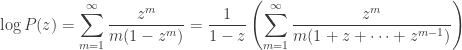
and it will turn out to be convenient to rearrange this a little: expanding this out gives
![\displaystyle \sum_{k=1}^{\infty} \sum_{m=1}^{\infty} \frac{z^{km}}{m}]()
and exchanging the order of summation gives
![\displaystyle \log P(z) = \sum_{m=1}^{\infty} \frac{z^m}{m (1 - z^m)} = \frac{1}{1 - z} \left( \sum_{m=1}^{\infty} \frac{z^m}{m(1 + z + \dots + z^{m-1})} \right)]() .
.
The point of writing ![\log P(z)]() in this way is to make the behavior as
in this way is to make the behavior as ![z \to 1^{-}]() very clear: we see that as
very clear: we see that as ![z \to 1^{-}]() ,
, ![\log P(z)]() approaches
approaches
![\displaystyle \frac{1}{1 - z} \sum_{m=1}^{\infty} \frac{1}{m^2} = \frac{\pi^2}{6(1 - z)}]() .
.
It turns out that as ![n \to \infty]() , the saddle point gets closer and closer to the essential singularity at
, the saddle point gets closer and closer to the essential singularity at ![z = 1]() . Near this singularity we may as well for the sake of convenience replace
. Near this singularity we may as well for the sake of convenience replace ![\log P(z)]() with
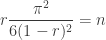
with ![\frac{\pi^2}{6(1 - z)}]() , which gives the approximate saddle point equation
, which gives the approximate saddle point equation
![\displaystyle r \frac{\pi^2}{6(1 - r)^2} = n]() .
.
This saddle point equation reinforces the idea that ![r]() is close to
is close to ![1]() : the only way to solve it in the interval
: the only way to solve it in the interval ![(0, 1)]() is to take something like
is to take something like ![r = 1 - \frac{C}{\sqrt{n}}]() , so we can ignore the
, so we can ignore the ![r]() factor, which gives the approximate saddle point
factor, which gives the approximate saddle point
![\displaystyle r = 1 - \frac{\pi}{\sqrt{6n}}]() .
.
and saddle point bound
![\displaystyle p(n) \le \frac{P(r)}{r^n}]() .
.
From here we need an upper bound on ![P(r)]() and a lower bound on
and a lower bound on ![r^n]() to get an upper bound on
to get an upper bound on ![p(n)]() . Edit, 12/12/16: As Akshaj explains in the comments, the argument that was previously here regarding the lower bound on
. Edit, 12/12/16: As Akshaj explains in the comments, the argument that was previously here regarding the lower bound on ![r^n]() was incorrect. Akshaj’s argument involving the Taylor series of log gives
was incorrect. Akshaj’s argument involving the Taylor series of log gives
![\displaystyle \left( 1 - \frac{\pi}{\sqrt{6n}} \right)^n \ge \exp \left( - \pi \sqrt{ \frac{n}{6} } - \frac{\pi^2}{12} + O \left( \frac{1}{\sqrt{n}} \right) \right).]()
As for the upper bound on ![P(r)]() , if
, if ![r \in (0, 1)]() then
then ![r^n \le r^k]() for
for ![0 \le k \le n-1]() , hence
, hence
![\displaystyle nr^n \le 1 + r + \dots + r^{n-1} \Leftrightarrow \frac{r^n}{1 + r + \dots + r^{n-1}} \le \frac{1}{n}]()
from which we conclude that
![\displaystyle \log P(r) \le \frac{1}{1 - r} \frac{\pi^2}{6} = \pi \sqrt{ \frac{n}{6} }]()
and hence that
![\displaystyle p(n) \le \frac{P(r)}{r^n} \le \exp \left( \pi \sqrt{ \frac{2n}{3}} + \frac{\pi^2}{12} + O \left( \frac{1}{\sqrt{n}} \right) \right)]()
which is ![O(n)]() off from the true answer.
off from the true answer.
Of course, without knowing a better method that in fact gives the true answer, we have no way of independently verifying that the saddle point bounds are as close as we’ve claimed they are. We need a more powerful idea to turn these bounds into asymptotics and recover our factors of ![O(n^a)]() .
.
Hardy’s approach
In the eighth of Hardy’s twelve lectures on Ramanujan’s work, he describes a more down-to-earth way to guess that
![\displaystyle \log p(n) \approx \pi \sqrt{ \frac{2n}{3} }]()
starting from the approximation
![\displaystyle \log P(z) \approx \frac{\pi^2}{6(1 - z)}]() .
.
as ![z \to 1^{-}]() . He first observes that
. He first observes that ![p(n)]() must grow faster than a polynomial but slower than an exponential: if
must grow faster than a polynomial but slower than an exponential: if ![p(n)]() grew like a polynomial then
grew like a polynomial then ![P(z)]() would have a pole of finite order at
would have a pole of finite order at ![z = 1]() , whereas if
, whereas if ![p(n)]() grew like an exponential then
grew like an exponential then ![P(z)]() would have a singularity closer to the origin. Hence, in Hardy’s words, it is “natural to conjecture” that
would have a singularity closer to the origin. Hence, in Hardy’s words, it is “natural to conjecture” that
![\displaystyle p(n) \approx \exp (A n^a)]()
for some ![A > 0]() and some
and some ![a \in (0, 1)]() . From here he more or less employs a saddle point bound in reverse, estimating
. From here he more or less employs a saddle point bound in reverse, estimating
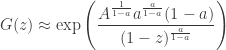
![\displaystyle G(z) = \sum \exp (A n^a) ;z^n]()
based on the size of its largest term. It’s convenient to write ![z = \exp(-t)]() so that this sum can be rewritten
so that this sum can be rewritten
![\displaystyle G(z) = \sum \exp (A n^a - nt)]()
so that, differentiating in ![n]() , we see that the maximum occurs when
, we see that the maximum occurs when ![A a n^{a-1} = t]() . We want to turn this into an estimate for
. We want to turn this into an estimate for ![G(z)]() involving only
involving only ![A, a, z]() , so we want to eliminate
, so we want to eliminate ![n]() and use the approximation
and use the approximation ![t \approx 1 - z]() , valid as
, valid as ![z \to 1^{-}]() . This gives
. This gives
![\displaystyle n = \left( \frac{t}{Aa} \right)^{ \frac{1}{a-1} } = \left( \frac{Aa}{1 - z} \right)^{ \frac{1}{1-a} }]()
(keeping in mind that ![1 - a]() is positive), so that
is positive), so that
![\displaystyle A n^a = \frac{A^{ \frac{1}{1-a} } a^{ \frac{a}{1-a} }}{(1 - z)^{ \frac{a}{1-a} } }]()
and
![\displaystyle ny = \frac{ A^{ \frac{1}{1-a} } a^{ \frac{1}{1-a} } }{(1 - z)^{ \frac{a}{1-a} }}]()
which altogether gives (again, approximating ![G(z)]() by its largest term)
by its largest term)
![\displaystyle G(z) \approx \exp \left( \frac{ A^{\frac{1}{1-a}} a^{ \frac{a}{1-a} } (1 - a) }{ (1 - z)^{ \frac{a}{1-a} } } \right)]()
for ![z \to 1^{-}]() . Matching this up with
. Matching this up with ![\exp \left( \frac{\pi^2}{6(1 - z)} \right)]() gives
gives ![a = \frac{1}{2}]() and
and
![\displaystyle \frac{A^2}{4} = \frac{\pi^2}{6}]()
hence ![A = \pi \sqrt{ \frac{2}{3} }]() .
.
The saddle point method
The saddle point bound, although surprisingly informative, uses very little of the information provided by the Cauchy integral formula. We ought to be able to do a lot better by picking a contour ![\gamma]() to integrate over such that we can, by analyzing the contour integral more closely, bound the contour integral
to integrate over such that we can, by analyzing the contour integral more closely, bound the contour integral
![\displaystyle a_n = \frac{1}{2\pi i} \oint_{\gamma} \frac{A(z)}{z^{n+1}} \, dz]()
more carefully than just by the “trivial” bound ![\ell(\gamma) \sup_{z \in \gamma} \left| \frac{A(z)}{z^{n+1}} \right|]() .
.
From here we’ll still be looking at saddle points, but more carefully, as follows. Ignoring the length factor ![\ell(\gamma)]() in the trivial bound, if we try to minimize
in the trivial bound, if we try to minimize ![\sup_{z \in \gamma} \left| \frac{A(z)}{z^{n+1}} \right|]() we’ll end up at a saddle point
we’ll end up at a saddle point ![r]() of
of ![\frac{A(z)}{z^{n+1}}]() (so we get a point very slightly different from above, where we used a saddle point of
(so we get a point very slightly different from above, where we used a saddle point of ![\frac{A(z)}{z^n}]() ). Depending on the geometry of the locations of the zeroes, poles, and saddle points of
). Depending on the geometry of the locations of the zeroes, poles, and saddle points of ![\frac{A(z)}{z^{n+1}}]() , we can hope to choose
, we can hope to choose ![\gamma]() to be a contour that passes through this saddle point
to be a contour that passes through this saddle point ![r]() in such a way that
in such a way that ![\left| \frac{A(z)}{z^{n+1}} \right|]() is in fact maximized at
is in fact maximized at ![z = r]() . This means that
. This means that ![\gamma]() should enter and exit the “saddle” around the saddle point in the direction of steepest descent from the saddle point.
should enter and exit the “saddle” around the saddle point in the direction of steepest descent from the saddle point.
If we pick ![\gamma]() carefully, and
carefully, and ![A(z)]() has certain nice properties, we can furthermore hope that
has certain nice properties, we can furthermore hope that
- the contour integral over a small arc (in terms of the circle method, the “major arc”) is easy to approximate (usually by a Gaussian integral), and
- the contour integral over everything else (in terms of the circle method, the “minor arc”) is small enough that it’s easy to bound.
The Gaussian integrals that often appear when integrating over the major arc are responsible for the factors of ![O(\sqrt{n})]() we lost above.
we lost above.
Let’s see how this works in the case of the factorials, where ![A(z) = e^z]() . The function
. The function ![\frac{e^z}{z^{n+1}}]() has a unique saddle point at
has a unique saddle point at ![n+1]() , but to simplify the computation we’ll take
, but to simplify the computation we’ll take ![r = n]() as before. We’ll take
as before. We’ll take ![\gamma]() to be the circle of radius
to be the circle of radius ![r = n]() , which gives a contour integral which can be rewritten in polar coordinates as
, which gives a contour integral which can be rewritten in polar coordinates as
![\displaystyle \frac{1}{n!} = \frac{1}{2\pi} \int_{-\pi}^{\pi} \frac{e^{n e^{i \theta}}}{n^n e^{i n \theta}} \, d \theta = \frac{e^n}{2 \pi n^n} \int_{-\pi}^{\pi} e^{n (e^{i \theta} - 1) - i n \theta} \, d \theta]() .
.
This integral can also be thought of as coming from computing the Fourier coefficients of a suitable Fourier series. Write the integrand as ![e^{f(\theta) + i g(\theta)}]() , so that
, so that
![\displaystyle f(\theta) = n (\cos \theta - 1), g(\theta) = n (\sin \theta - \theta)]() .
.
![g(\theta)]() only controls the phase of the integrand, and since it doesn’t vary much (it grows like
only controls the phase of the integrand, and since it doesn’t vary much (it grows like ![O(n \theta^3)]() for small
for small ![\theta]() ) we’ll be able to ignore it.
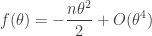
) we’ll be able to ignore it. ![f(\theta)]() controls the absolute value of the integrand and so is much more important. For small values of
controls the absolute value of the integrand and so is much more important. For small values of ![\theta]() we have
we have
![\displaystyle f(\theta) = -\frac{n \theta^2}{2} + O(\theta^4)]()
so from here we can try to break up the integral into a “major arc” where ![\theta \in (-\delta, \delta)]() for some small (where the meaning of “small” depends on
for some small (where the meaning of “small” depends on ![n]() )
) ![\delta]() and a “minor arc” consisting of the other values of
and a “minor arc” consisting of the other values of ![\theta]() , and try to show both the integral over the major arc is well approximated by the Gaussian integral
, and try to show both the integral over the major arc is well approximated by the Gaussian integral
![\displaystyle \int_{-\infty}^{\infty} e^{- \frac{n \theta^2}{2} } \, d \theta = \sqrt{ \frac{2\pi}{n} }]()
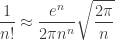
and that the integral over the minor arc is negligible compared to this. This can be done, and the details are in Flajolet and Sedgewick (who take ![\delta = n^{-2/5}]() ); ignoring all the details, the conclusion is that
); ignoring all the details, the conclusion is that
![\displaystyle \frac{1}{n!} \approx \frac{e^n}{2 \pi n^n} \sqrt{ \frac{2\pi}{n} }]()
and hence that
![\displaystyle n! \approx \sqrt{2 \pi n} \frac{n^n}{e^n}]()
which is exactly Stirling’s approximation. This computation also has a probabilistic interpretation: it says that the probability that a Poisson random variable with rate ![n]() takes its mean value
takes its mean value ![n]() is asymptotically
is asymptotically ![\frac{1}{\sqrt{2\pi n}}]() , which can be viewed as a corollary of the central limit theorem, since such a Poisson random variable is a sum of
, which can be viewed as a corollary of the central limit theorem, since such a Poisson random variable is a sum of ![n]() independent Poisson random variables with rate
independent Poisson random variables with rate ![1]() .
.
In general we’ll again find that, under suitable hypotheses, we can approximate the major arc integral by a Gaussian integral (using the same strategy as above) and bound the minor arc integral to show that it’s negligible. This gives the following:
Theorem (saddle point approximation): Under suitable hypotheses, if ![A(z) = \sum a_n z^n]() and
and ![\frac{A(z)}{z^{n+1}} = e^{f(z)}]() , let
, let ![r]() be a saddle point of
be a saddle point of ![\left| \frac{A(z)}{z^{n+1}} \right|]() , so that
, so that ![f'(r) = 0]() . Then, as
. Then, as ![n \to \infty]() , we have
, we have
![\displaystyle a_n \approx \frac{e^{f(r)}}{\sqrt{2 \pi f''(r)}}]() .
.
Directly applying this theorem to the partition function is difficult because of the difficulty of bounding what happens on the minor arc. ![P(z)]() has essential singularities on a dense subset of the unit circle, and delicate analysis has to be done to describe the contributions of these singularities (or more precisely, of saddle points near these singularities); the circle method used by Hardy and Ramanujan to prove the asymptotic formula accomplishes this by choosing the contour
has essential singularities on a dense subset of the unit circle, and delicate analysis has to be done to describe the contributions of these singularities (or more precisely, of saddle points near these singularities); the circle method used by Hardy and Ramanujan to prove the asymptotic formula accomplishes this by choosing the contour ![\gamma]() very carefully and then using modularity properties of
very carefully and then using modularity properties of ![P(z)]() (which is closely related to the eta function).
(which is closely related to the eta function).
We will completely ignore these difficulties and pretend that only the contribution from the (saddle point near the) essential singularity at ![z = 1]() matters to the leading term. Even ignoring the minor arc, to make use of the saddle point approximation requires that we know the asymptotics of
matters to the leading term. Even ignoring the minor arc, to make use of the saddle point approximation requires that we know the asymptotics of ![P(z)]() as
as ![z \to 1^{-}]() in more detail than we do right now.
in more detail than we do right now.
Unfortunately there does not seem to be a really easy way to do this; Hardy’s approach uses the modular properties of the eta function, while Flajolet and Sedgewick use Mellin transforms. So at this point we’ll just quote without proof the asymptotic we need from Flajolet and Sedgewick, up to the accuracy we need, namely
![\displaystyle \log P(z) = \frac{\pi^2}{6(1 - z)} + \frac{1}{2} \log (1 - z) + O(1)]() .
.
Although this changes the location of the saddle point slightly, for ease of computation (and because it will lose us at worst multiplicative factors in the end) we’ll continue to work with the same approximate saddle point
![\displaystyle r = 1 - \frac{\pi}{\sqrt{6n}}]()
as before. The saddle point approximation differs from the saddle point bound ![\exp \left( \pi \sqrt{ \frac{2n}{3}} \right)]() we established earlier in two ways: first, the introduction of the
we established earlier in two ways: first, the introduction of the ![\frac{1}{2} \log (1 - z)]() term contributes a factor of
term contributes a factor of
![\displaystyle \sqrt{1 - r} = \Theta \left( n^{- \frac{1}{4}} \right)]()
and second, the introduction of the denominator ![\sqrt{2\pi f''(r)}]() contributes another factor, which we approximate as follows. We have
contributes another factor, which we approximate as follows. We have
![\displaystyle f(z) \approx \frac{\pi^2}{6(1 - z)} + \frac{1}{2} \log (1 - z) - (n+1) \log z]()
and hence
![\displaystyle f'(z) \approx \frac{\pi^2}{6(1 - z)^2} - \frac{1}{2(1 - z)} - \frac{n+1}{z}]()
so that
![\displaystyle f''(z) \approx \frac{\pi^2}{3(1 - z)^3} - \frac{1}{2(1 - z)^2} + \frac{n+1}{z^2}]()
which gives ![f''(r) = \Theta \left( n^{\frac{3}{2}} \right)]() (we actually know the multiplicative constant here, but it doesn’t matter because we already lost multiplicative constants when estimating
(we actually know the multiplicative constant here, but it doesn’t matter because we already lost multiplicative constants when estimating ![e^{f(r)}]() ) and hence
) and hence
![\displaystyle \sqrt{2\pi f''(r)} = \Theta \left( n^{\frac{3}{4}} \right)]() .
.
Altogether the saddle point approximation, up to a multiplicative constant, is
![\displaystyle p(n) = \Theta \left( \frac{1}{n} \exp \left( \pi \sqrt{\frac{2n}{3}} \right) \right)]() .
.